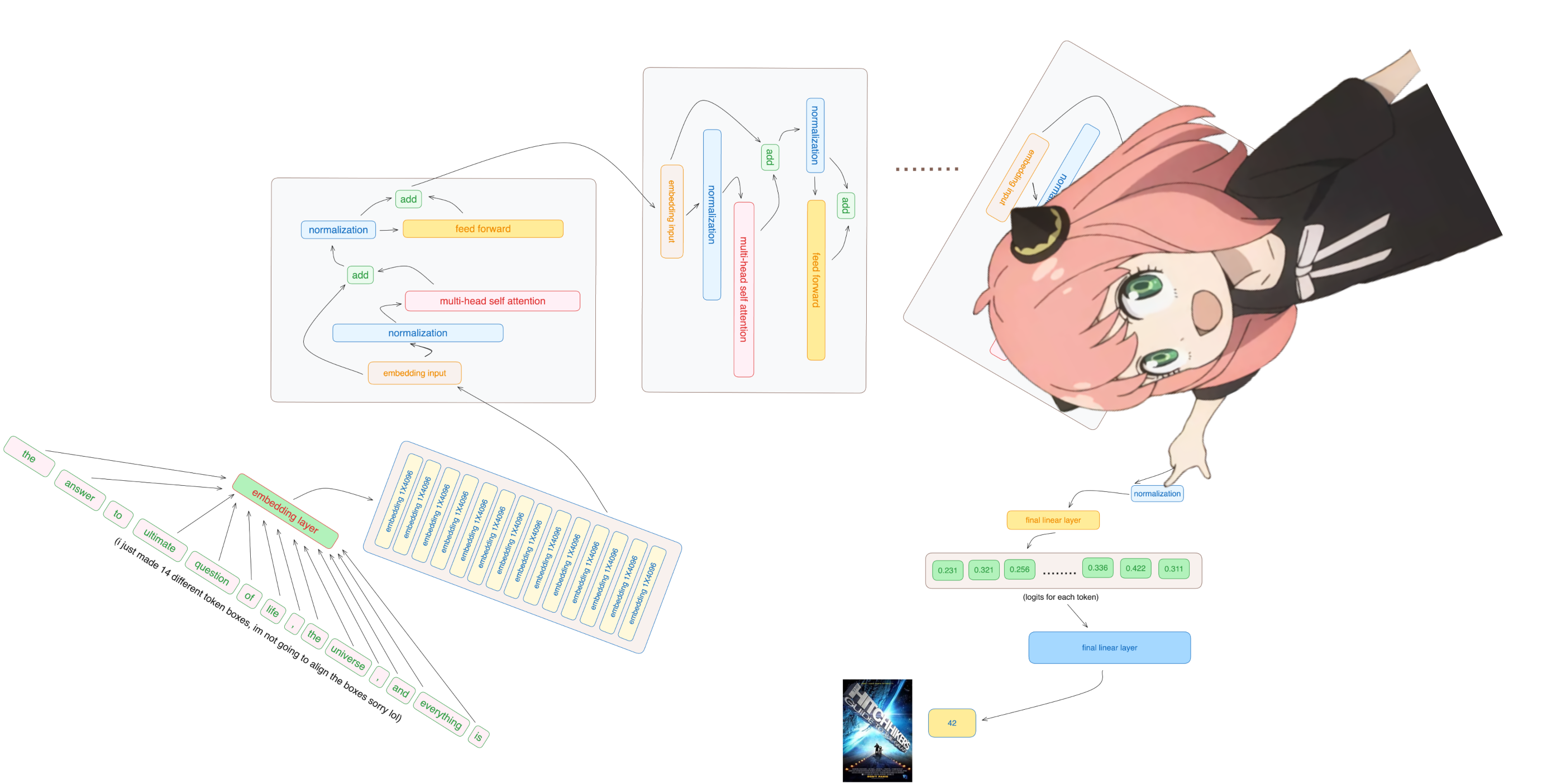
从头开始实现llama3

都说大模型是黑箱玄学，这次让我们打开黑箱，一起来探索它内部的世界。

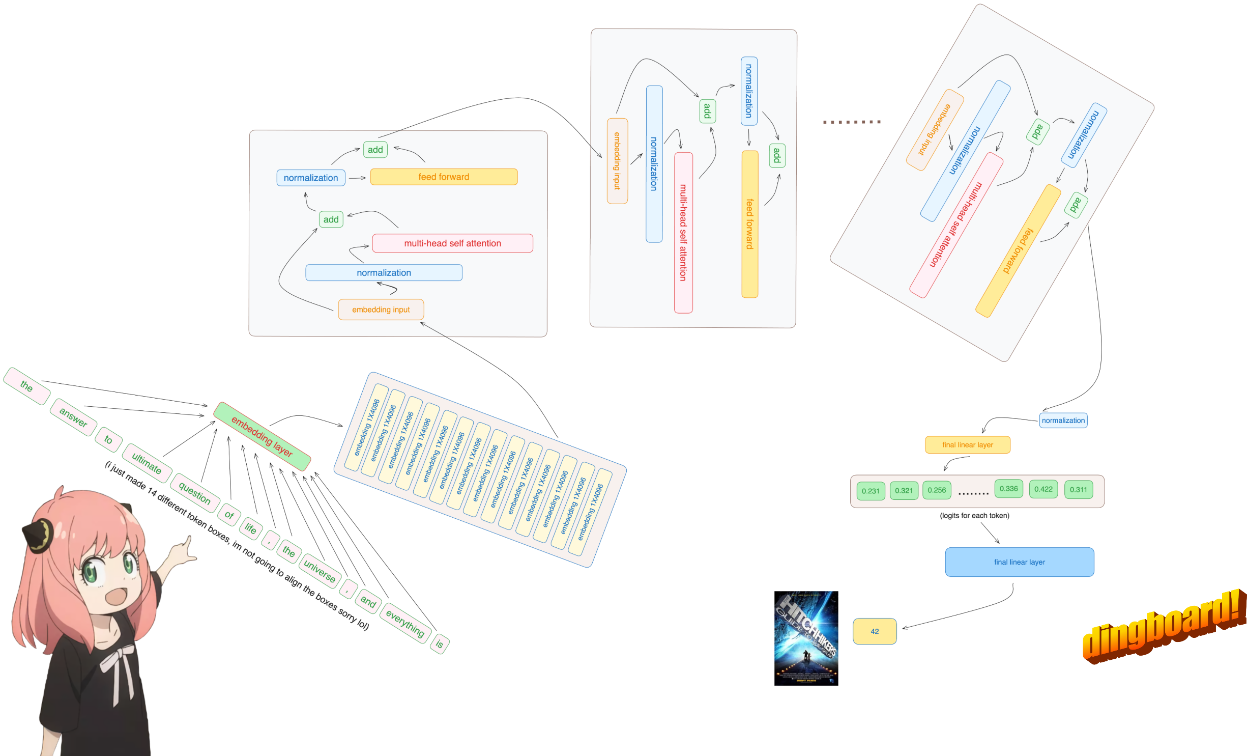
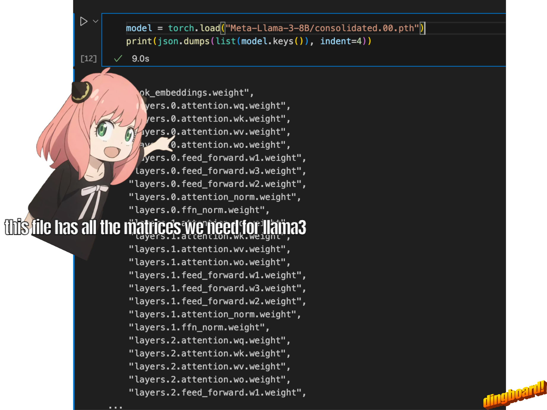
在这个文件中，我从头开始实现了 llama3，一次一个张量和矩阵乘法。另外，我将直接从Meta为 llama3 提供的模型文件加载张量，您需要在运行此文件之前下载权重。这是下载权重的官方链接：https://llama.meta.com/llama-downloads/

img

1.分词器（tokenizer）

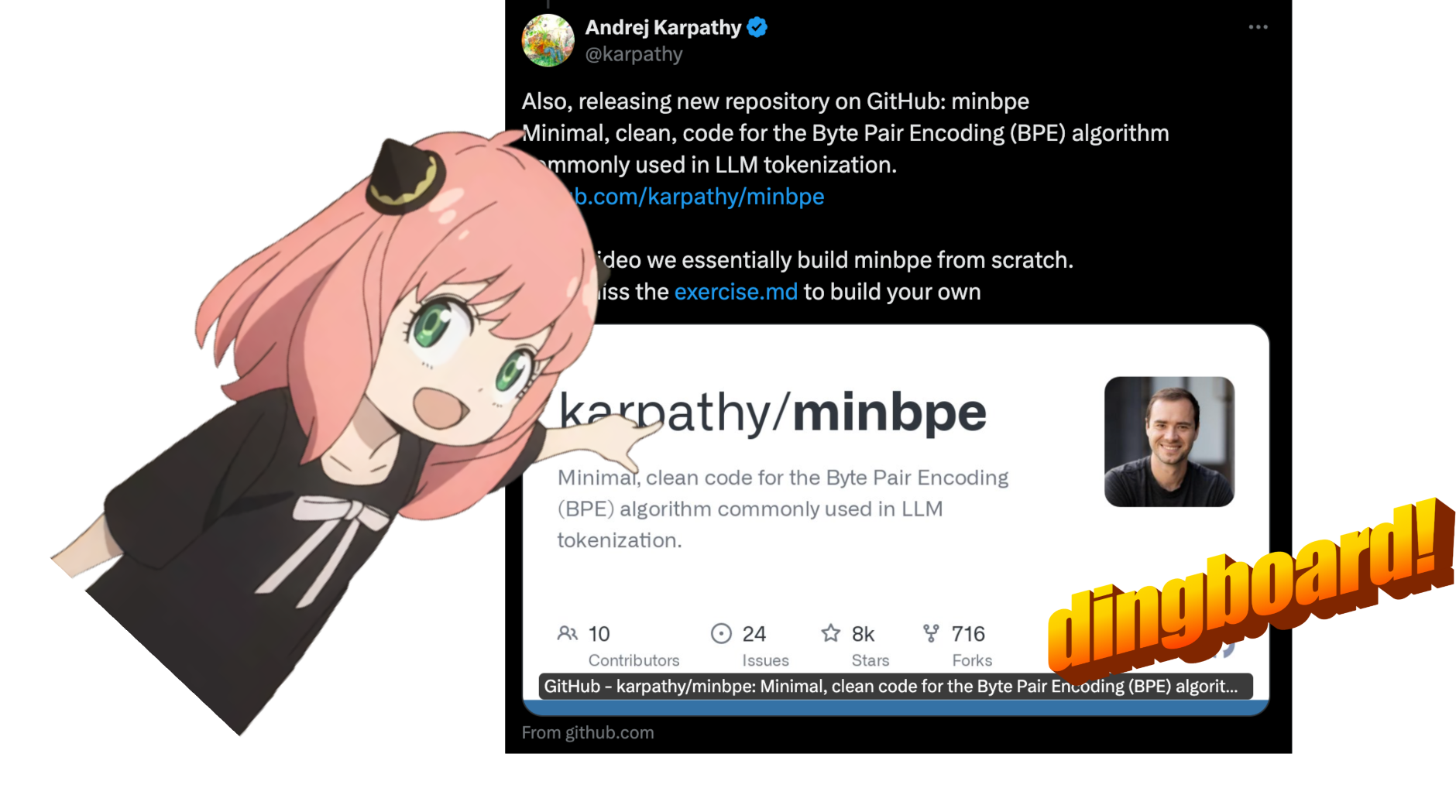
我不会实现 bpe tokenizer（但 andrej karpathy 有一个非常干净的实现） 他的实现链接：[https://github.com/karpathy/minbpe)

img

from pathlib import Path
import tiktoken
from tiktoken.load import load_tiktoken_bpe
import torch
import json
import matplotlib.pyplot as plt

tokenizer_path = "Meta-Llama-3-8B/tokenizer.model"
special_tokens = [
            "<|begin_of_text|>",
            "<|end_of_text|>",
            "<|reserved_special_token_0|>",
            "<|reserved_special_token_1|>",
            "<|reserved_special_token_2|>",
            "<|reserved_special_token_3|>",
            "<|start_header_id|>",
            "<|end_header_id|>",
            "<|reserved_special_token_4|>",
            "<|eot_id|>",  # end of turn
        ] + [f"<|reserved_special_token_{i}|>" for i in range(5, 256 - 5)]
mergeable_ranks = load_tiktoken_bpe(tokenizer_path)
tokenizer = tiktoken.Encoding(
    name=Path(tokenizer_path).name,
    pat_str=r"(?i:'s|'t|'re|'ve|'m|'ll|'d)|[^\r\n\p{L}\p{N}]?\p{L}+|\p{N}{1,3}| ?[^\s\p{L}\p{N}]+[\r\n]*|\s*[\r\n]+|\s+(?!\S)|\s+",
    mergeable_ranks=mergeable_ranks,
    special_tokens={token: len(mergeable_ranks) + i for i, token in enumerate(special_tokens)},
)

tokenizer.decode(tokenizer.encode("hello world!"))
'hello world!'

2.读取模型文件

通常，阅读本文取决于模型类的编写方式以及其中的变量名称。 但由于我们是从头开始实现 llama3，因此我们将一次读取一个张量文件。

img

model = torch.load("Meta-Llama-3-8B/consolidated.00.pth")
print(json.dumps(list(model.keys())[:20], indent=4))
[
    "tok_embeddings.weight",
    "layers.0.attention.wq.weight",
    "layers.0.attention.wk.weight",
    "layers.0.attention.wv.weight",
    "layers.0.attention.wo.weight",
    "layers.0.feed_forward.w1.weight",
    "layers.0.feed_forward.w3.weight",
    "layers.0.feed_forward.w2.weight",
    "layers.0.attention_norm.weight",
    "layers.0.ffn_norm.weight",
    "layers.1.attention.wq.weight",
    "layers.1.attention.wk.weight",
    "layers.1.attention.wv.weight",
    "layers.1.attention.wo.weight",
    "layers.1.feed_forward.w1.weight",
    "layers.1.feed_forward.w3.weight",
    "layers.1.feed_forward.w2.weight",
    "layers.1.attention_norm.weight",
    "layers.1.ffn_norm.weight",
    "layers.2.attention.wq.weight"
]
with open("Meta-Llama-3-8B/params.json", "r") as f:
    config = json.load(f)
config
{'dim': 4096,
 'n_layers': 32,
 'n_heads': 32,
 'n_kv_heads': 8,
 'vocab_size': 128256,
 'multiple_of': 1024,
 'ffn_dim_multiplier': 1.3,
 'norm_eps': 1e-05,
 'rope_theta': 500000.0}

我们使用此配置来推断有关模型的详细信息，例如

1. 该模型有 32 个transformer layers
2. 每个多头注意力块有 32 个头
3. 词汇大小等等

dim = config["dim"]
n_layers = config["n_layers"]
n_heads = config["n_heads"]
n_kv_heads = config["n_kv_heads"]
vocab_size = config["vocab_size"]
multiple_of = config["multiple_of"]
ffn_dim_multiplier = config["ffn_dim_multiplier"]
norm_eps = config["norm_eps"]
rope_theta = torch.tensor(config["rope_theta"])

将文本转换为标记（tokens）

这里我们使用 tiktoken （我认为是一个 openai 库）作为 tokenizer

img

prompt = "the answer to the ultimate question of life, the universe, and everything is "
tokens = [128000] + tokenizer.encode(prompt)
print(tokens)
tokens = torch.tensor(tokens)
prompt_split_as_tokens = [tokenizer.decode([token.item()]) for token in tokens]
print(prompt_split_as_tokens)
[128000, 1820, 4320, 311, 279, 17139, 3488, 315, 2324, 11, 279, 15861, 11, 323, 4395, 374, 220]
['<|begin_of_text|>', 'the', ' answer', ' to', ' the', ' ultimate', ' question', ' of', ' life', ',', ' the', ' universe', ',', ' and', ' everything', ' is', ' ']

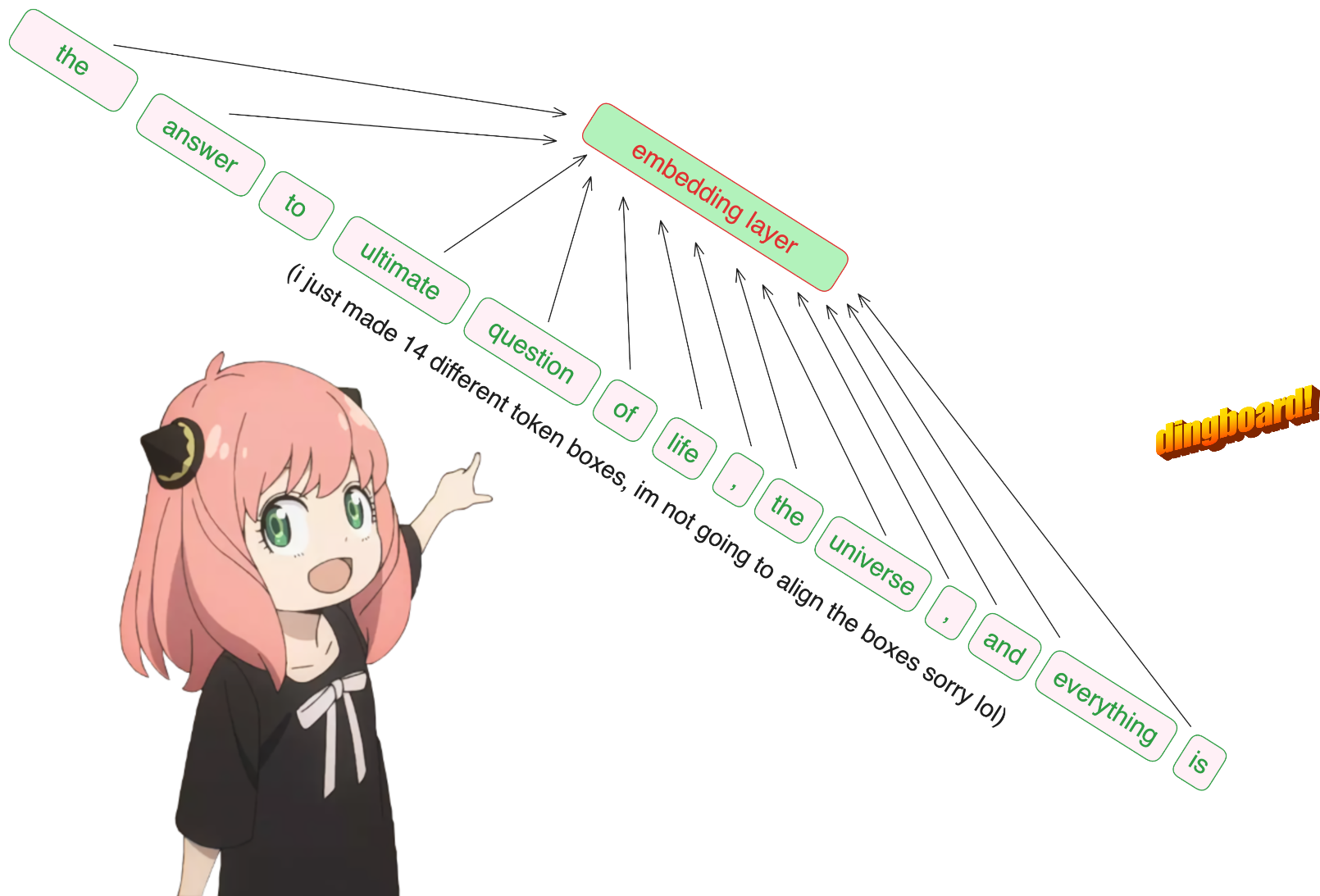
将标记转换为嵌入（embedding）

抱歉，但无论如何，这是代码库中我使用内置神经网络模块的唯一部分，因此我们的 [17x1] 标记现在是 [17x4096]，即长度为 4096 的 17 个嵌入（每个标记一个） 注意：跟踪形状，它让你更容易理解一切

img

embedding_layer = torch.nn.Embedding(vocab_size, dim)
embedding_layer.weight.data.copy_(model["tok_embeddings.weight"])
token_embeddings_unnormalized = embedding_layer(tokens).to(torch.bfloat16)
token_embeddings_unnormalized.shape
torch.Size([17, 4096])

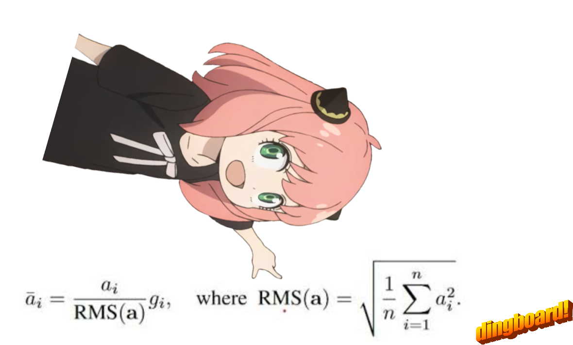
然后我们使用 rms 归一化对嵌入进行归一化

请注意，在这一步之后，形状不会改变，这些值只是需要记住的标准化内容，我们需要一个norm_eps（来自配置），因为我们不想意外地将rms设置为0并除以0，这里是公式：

img

# def rms_norm(tensor, norm_weights):
#     rms = (tensor.pow(2).mean(-1, keepdim=True) + norm_eps)**0.5
#     return tensor * (norm_weights / rms)
def rms_norm(tensor, norm_weights):
    return (tensor * torch.rsqrt(tensor.pow(2).mean(-1, keepdim=True) + norm_eps)) * norm_weights

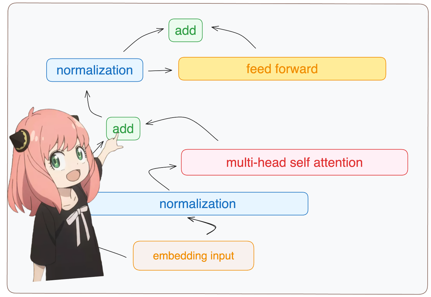
3.构建transformer的第一层

正常化

无论如何，你会看到我从模型字典访问layer.0（这是第一层），所以在标准化之后我们的形状仍然[17x4096]与嵌入相同但标准化

img

token_embeddings = rms_norm(token_embeddings_unnormalized, model["layers.0.attention_norm.weight"])
token_embeddings.shape
torch.Size([17, 4096])

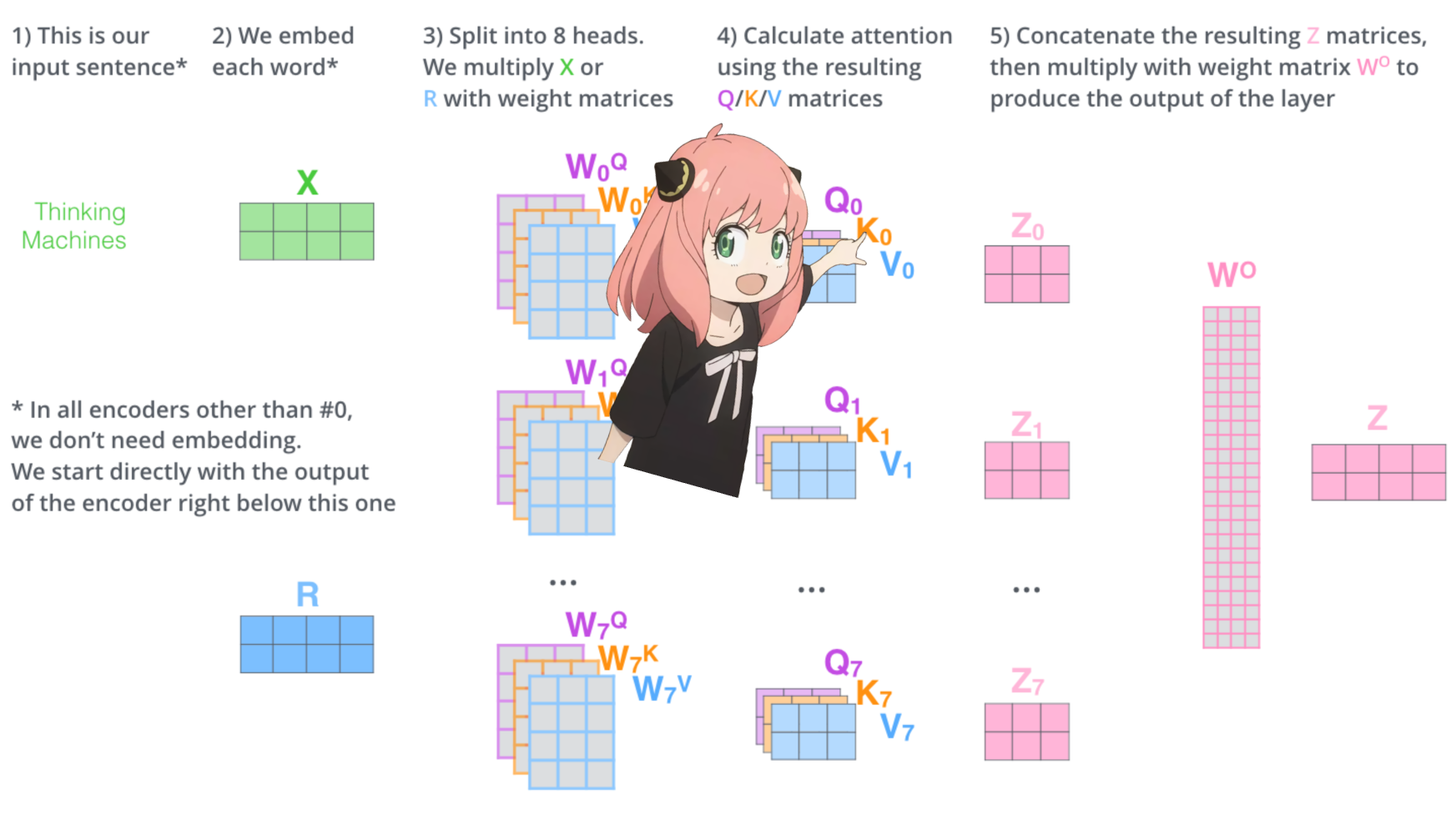
从头开始实施注意力

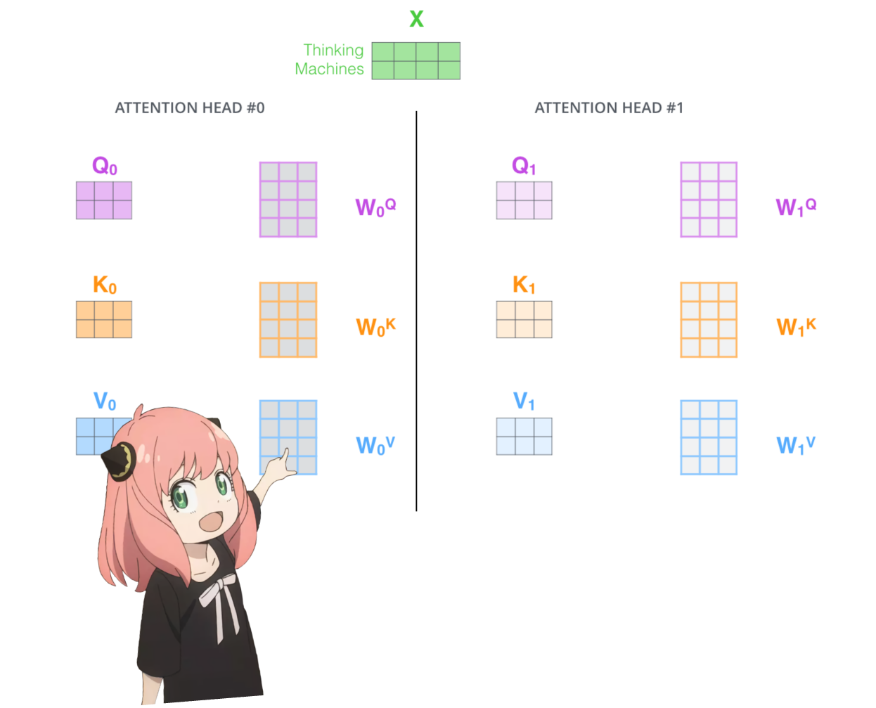
让我们加载transformer第一层的注意力头

img

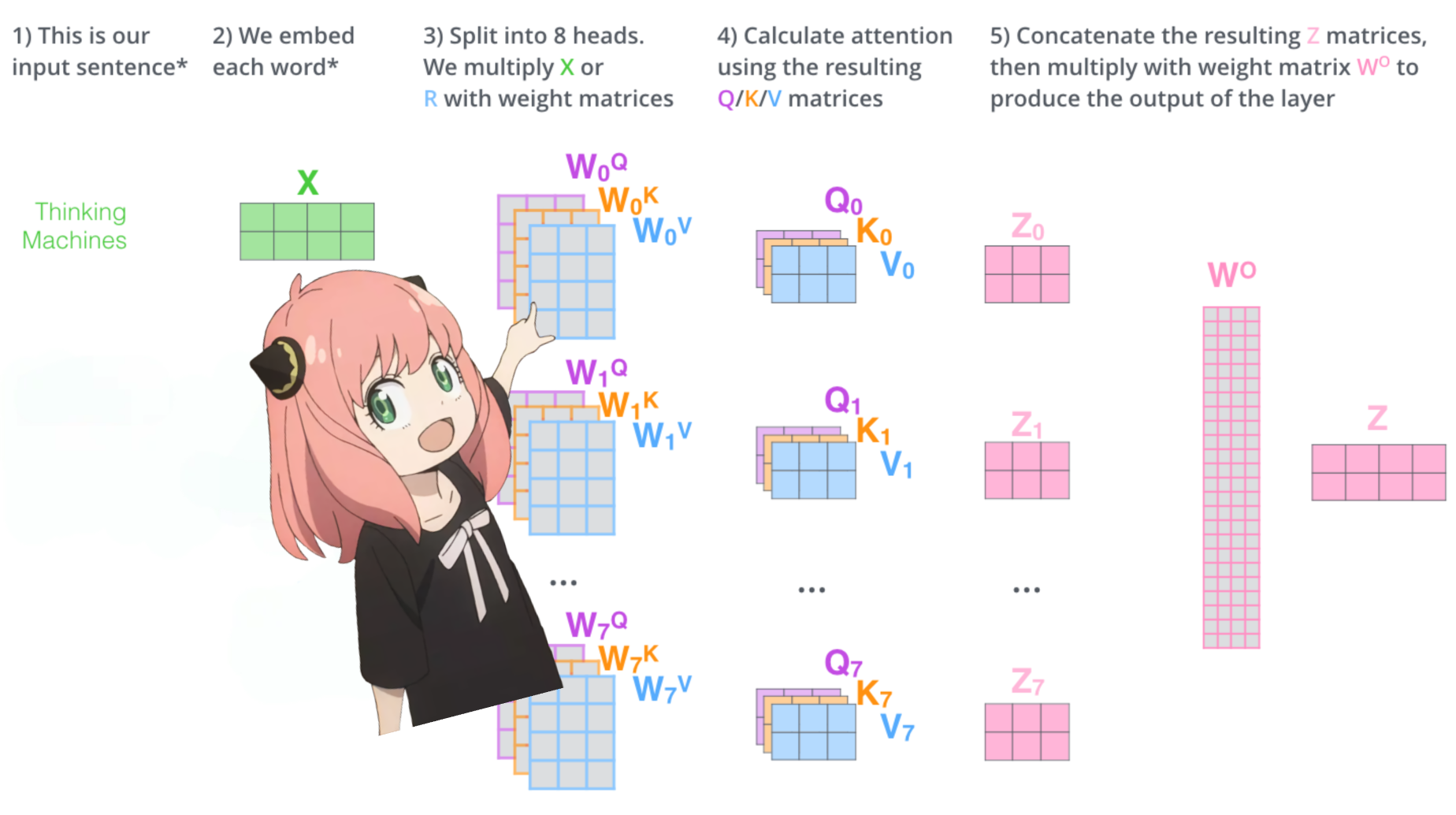
> 当我们从模型加载查询、键、值和输出向量时，我们注意到形状为 [4096x4096]、[1024x4096]、[1024x4096]、[4096x4096] > 乍一看这很奇怪，因为理想情况下我们想要每个 q ,k,v 和 o 分别代表每个头 > 代码的作者将它们捆绑在一起，因为它很容易，有助于并行化注意力头乘法。 > 我要打开所有东西...

print(
    model["layers.0.attention.wq.weight"].shape,
    model["layers.0.attention.wk.weight"].shape,
    model["layers.0.attention.wv.weight"].shape,
    model["layers.0.attention.wo.weight"].shape
)
torch.Size([4096, 4096]) torch.Size([1024, 4096]) torch.Size([1024, 4096]) torch.Size([4096, 4096])

展开查询

在下一节中，我们将从多个注意力头中解开查询，生成的形状为 [32x128x4096]，其中 32 是 llama3 中注意力头的数量，128 是查询向量的大小，4096 是令牌嵌入的大小

q_layer0 = model["layers.0.attention.wq.weight"]
head_dim = q_layer0.shape[0] // n_heads
q_layer0 = q_layer0.view(n_heads, head_dim, dim)
q_layer0.shape
torch.Size([32, 128, 4096])

我要实现第一层的第一个头

这里我访问第一层的查询权重矩阵第一个头，这个查询权重矩阵的大小是[128x4096]

q_layer0_head0 = q_layer0[0]
q_layer0_head0.shape
torch.Size([128, 4096])

我们现在将查询权重与令牌嵌入相乘，以接收令牌的查询

在这里你可以看到结果的形状是 [17x128]，这是因为我们有 17 个标记，每个标记都有一个 128 长度的查询。

img

q_per_token = torch.matmul(token_embeddings, q_layer0_head0.T)
q_per_token.shape
torch.Size([17, 128])

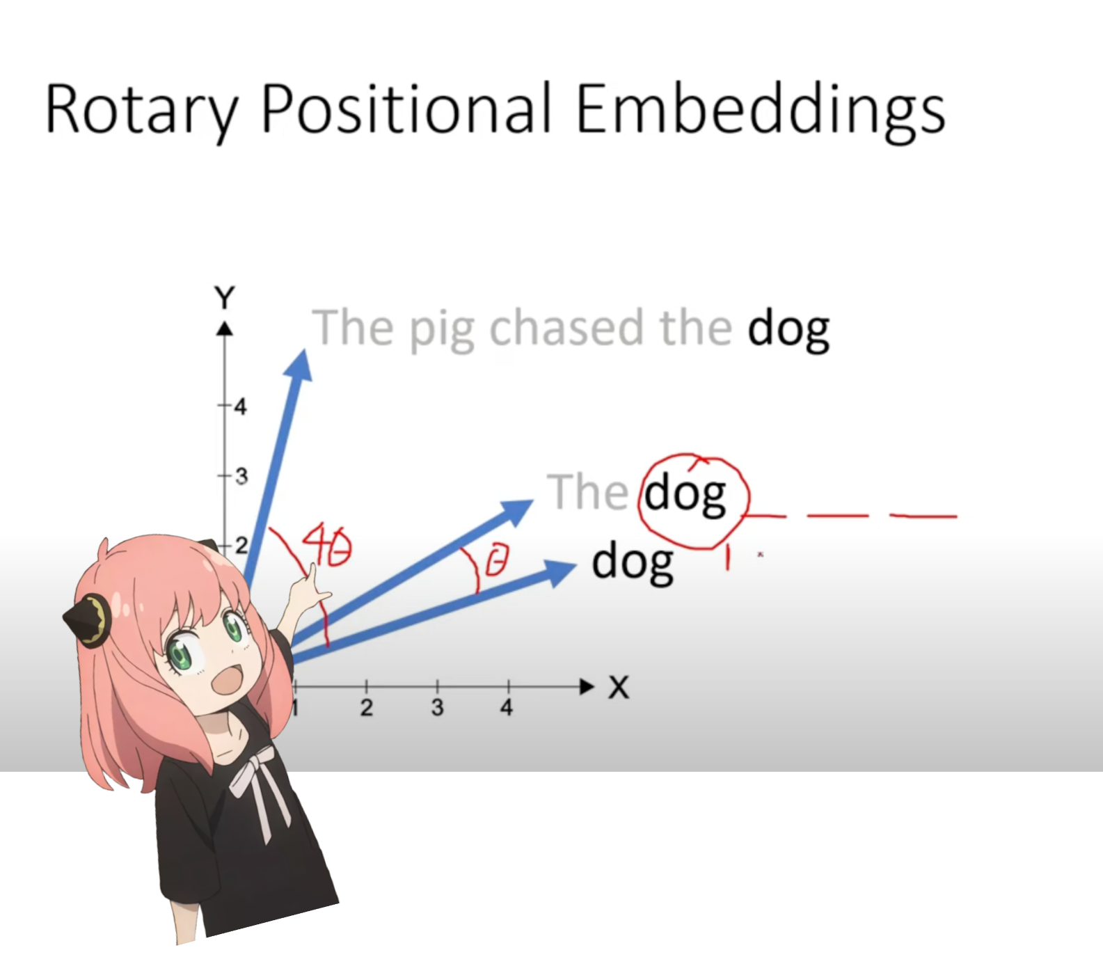
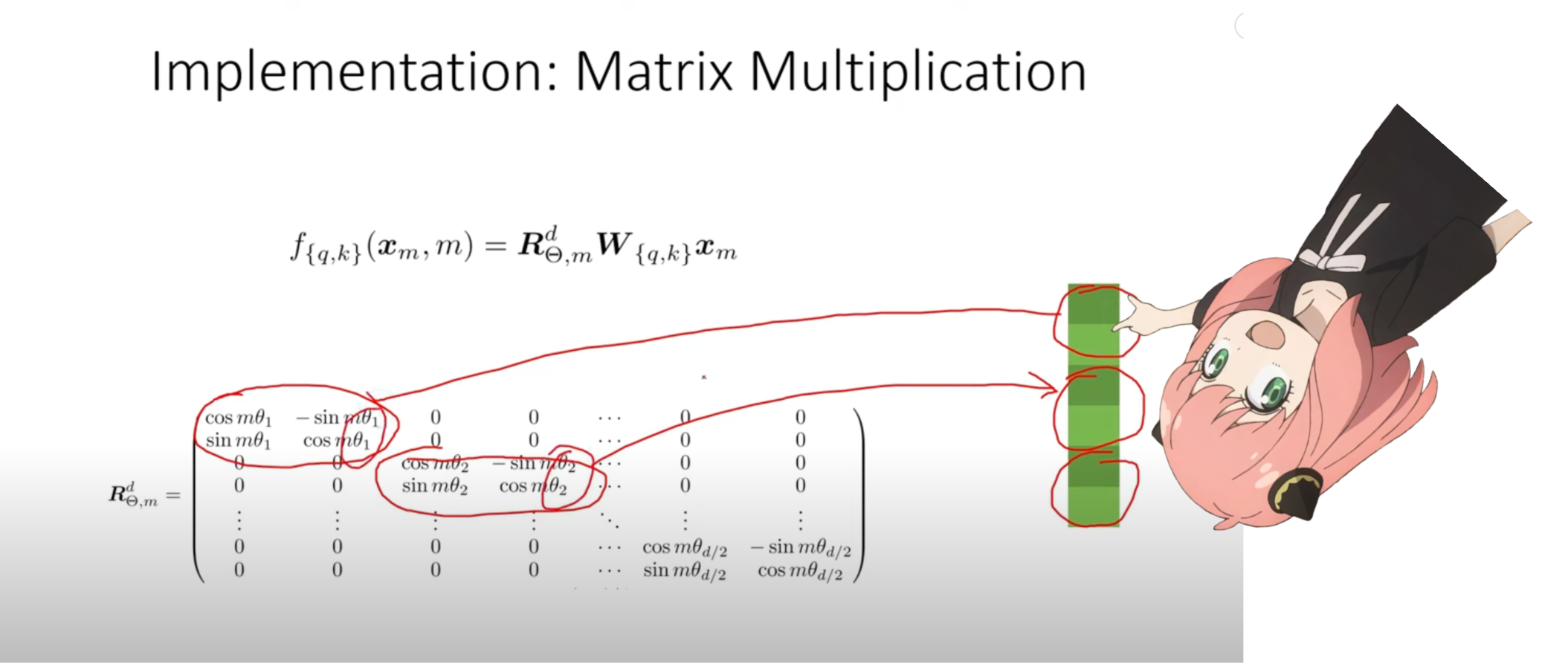
定位编码

我们现在处于这样一个阶段：提示中的每个标记都有一个查询向量，但如果你仔细想想——单独的查询向量不知道提示中的位置。 查询：“生命、宇宙和一切的终极问题的答案是” 在我们的提示中我们已经使用了“the”三次，我们需要所有 3 个“the”标记的查询向量具有不同的查询向量（每个大小 [1x128]）基于它们在查询中的位置。我们使用 RoPE（旋转位置嵌入）执行这些旋转。

RoPE

观看此视频（这就是我观看的）以理解数学。 https://www.youtube.com/watch?v=o29P0Kpobz0&t=530s

img

q_per_token_split_into_pairs = q_per_token.float().view(q_per_token.shape[0], -1, 2)
q_per_token_split_into_pairs.shape
torch.Size([17, 64, 2])

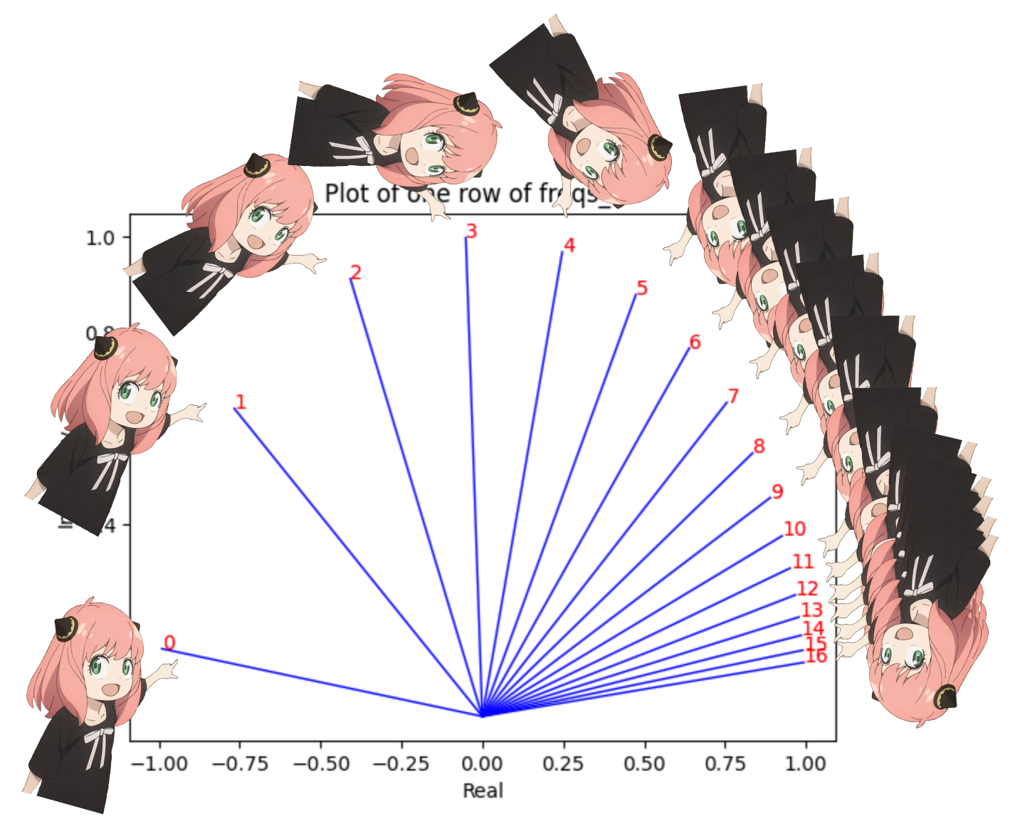
在上面的步骤中，我们将查询向量分成对，我们对每对应用旋转角度偏移！ 我们现在有一个大小为 [17x64x2] 的向量，这是针对提示中的每个标记将 128 个长度的查询分为 64 对！这 64 对中的每一对都将旋转 m*(theta)，其中 m 是我们旋转查询的标记的位置！

img

使用复数的点积来旋转向量

img

zero_to_one_split_into_64_parts = torch.tensor(range(64))/64
zero_to_one_split_into_64_parts
tensor([0.0000, 0.0156, 0.0312, 0.0469, 0.0625, 0.0781, 0.0938, 0.1094, 0.1250,
        0.1406, 0.1562, 0.1719, 0.1875, 0.2031, 0.2188, 0.2344, 0.2500, 0.2656,
        0.2812, 0.2969, 0.3125, 0.3281, 0.3438, 0.3594, 0.3750, 0.3906, 0.4062,
        0.4219, 0.4375, 0.4531, 0.4688, 0.4844, 0.5000, 0.5156, 0.5312, 0.5469,
        0.5625, 0.5781, 0.5938, 0.6094, 0.6250, 0.6406, 0.6562, 0.6719, 0.6875,
        0.7031, 0.7188, 0.7344, 0.7500, 0.7656, 0.7812, 0.7969, 0.8125, 0.8281,
        0.8438, 0.8594, 0.8750, 0.8906, 0.9062, 0.9219, 0.9375, 0.9531, 0.9688,
        0.9844])
freqs = 1.0 / (rope_theta ** zero_to_one_split_into_64_parts)
freqs
tensor([1.0000e+00, 8.1462e-01, 6.6360e-01, 5.4058e-01, 4.4037e-01, 3.5873e-01,
        2.9223e-01, 2.3805e-01, 1.9392e-01, 1.5797e-01, 1.2869e-01, 1.0483e-01,
        8.5397e-02, 6.9566e-02, 5.6670e-02, 4.6164e-02, 3.7606e-02, 3.0635e-02,
        2.4955e-02, 2.0329e-02, 1.6560e-02, 1.3490e-02, 1.0990e-02, 8.9523e-03,
        7.2927e-03, 5.9407e-03, 4.8394e-03, 3.9423e-03, 3.2114e-03, 2.6161e-03,
        2.1311e-03, 1.7360e-03, 1.4142e-03, 1.1520e-03, 9.3847e-04, 7.6450e-04,
        6.2277e-04, 5.0732e-04, 4.1327e-04, 3.3666e-04, 2.7425e-04, 2.2341e-04,
        1.8199e-04, 1.4825e-04, 1.2077e-04, 9.8381e-05, 8.0143e-05, 6.5286e-05,
        5.3183e-05, 4.3324e-05, 3.5292e-05, 2.8750e-05, 2.3420e-05, 1.9078e-05,
        1.5542e-05, 1.2660e-05, 1.0313e-05, 8.4015e-06, 6.8440e-06, 5.5752e-06,
        4.5417e-06, 3.6997e-06, 3.0139e-06, 2.4551e-06])
freqs_for_each_token = torch.outer(torch.arange(17), freqs)
freqs_cis = torch.polar(torch.ones_like(freqs_for_each_token), freqs_for_each_token)
freqs_cis.shape

# viewing tjhe third row of freqs_cis
value = freqs_cis[3]
plt.figure()
for i, element in enumerate(value[:17]):
    plt.plot([0, element.real], [0, element.imag], color='blue', linewidth=1, label=f"Index: {i}")
    plt.annotate(f"{i}", xy=(element.real, element.imag), color='red')
plt.xlabel('Real')
plt.ylabel('Imaginary')
plt.title('Plot of one row of freqs_cis')
plt.show()

img

现在我们对每个标记（token）的查询元素都有一个复数（角度变化向量）

我们可以将查询（我们分成对的查询）转换为复数，然后进行点积以根据位置诚实旋转查询，这想想就很美好:)

q_per_token_as_complex_numbers = torch.view_as_complex(q_per_token_split_into_pairs)
q_per_token_as_complex_numbers.shape
torch.Size([17, 64])
q_per_token_as_complex_numbers_rotated = q_per_token_as_complex_numbers * freqs_cis
q_per_token_as_complex_numbers_rotated.shape
torch.Size([17, 64])

得到旋转向量后

我们可以通过再次将复数视为实数来返回成对的查询

q_per_token_split_into_pairs_rotated = torch.view_as_real(q_per_token_as_complex_numbers_rotated)
q_per_token_split_into_pairs_rotated.shape
torch.Size([17, 64, 2])

旋转的对现在被合并，我们现在有一个新的查询向量（旋转查询向量），其形状为 [17x128]，其中 17 是标记的数量，128 是查询向量的暗度

q_per_token_rotated = q_per_token_split_into_pairs_rotated.view(q_per_token.shape)
q_per_token_rotated.shape
torch.Size([17, 128])

键（几乎与查询相同）

img

我太懒了，所以我不会对键进行数学计算，你需要记住的唯一事情是： > 键也生成维度 128 的键向量 > 键的权重数量只有 1/4查询，这是因为键的权重一次在 4 个头之间共享，为了减少需要的计算数量 > 键也会旋转以添加位置信息，就像查询一样，原因相同

k_layer0 = model["layers.0.attention.wk.weight"]
k_layer0 = k_layer0.view(n_kv_heads, k_layer0.shape[0] // n_kv_heads, dim)
k_layer0.shape
torch.Size([8, 128, 4096])
k_layer0_head0 = k_layer0[0]
k_layer0_head0.shape
torch.Size([128, 4096])
k_per_token = torch.matmul(token_embeddings, k_layer0_head0.T)
k_per_token.shape
torch.Size([17, 128])
k_per_token_split_into_pairs = k_per_token.float().view(k_per_token.shape[0], -1, 2)
k_per_token_split_into_pairs.shape
torch.Size([17, 64, 2])
k_per_token_as_complex_numbers = torch.view_as_complex(k_per_token_split_into_pairs)
k_per_token_as_complex_numbers.shape
torch.Size([17, 64])
k_per_token_split_into_pairs_rotated = torch.view_as_real(k_per_token_as_complex_numbers * freqs_cis)
k_per_token_split_into_pairs_rotated.shape
torch.Size([17, 64, 2])
k_per_token_rotated = k_per_token_split_into_pairs_rotated.view(k_per_token.shape)
k_per_token_rotated.shape
torch.Size([17, 128])

在此阶段，现在每个标记都有查询和键的旋转值。

img

现在每个查询和键的形状都是 [17x128]。

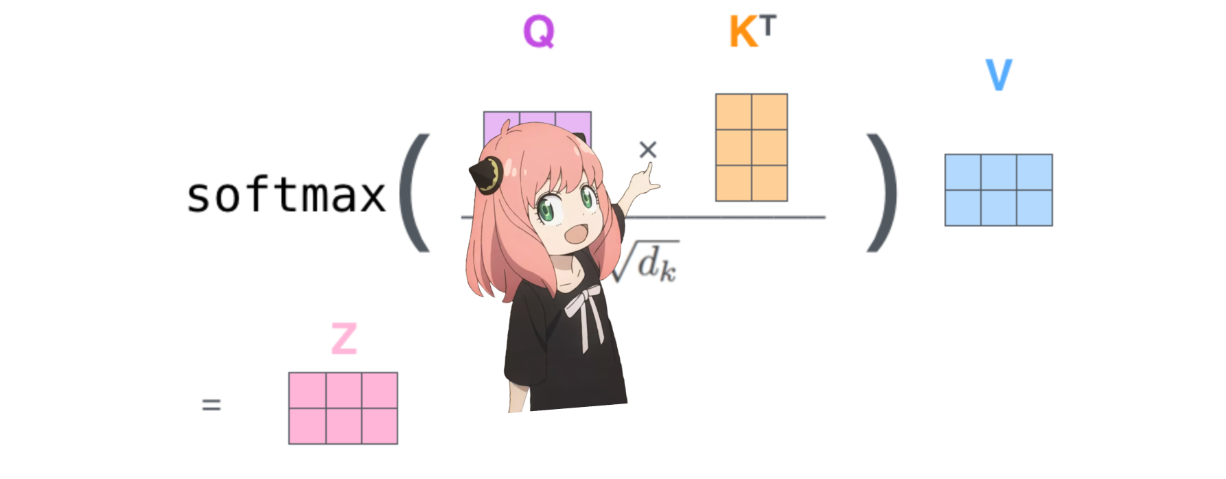
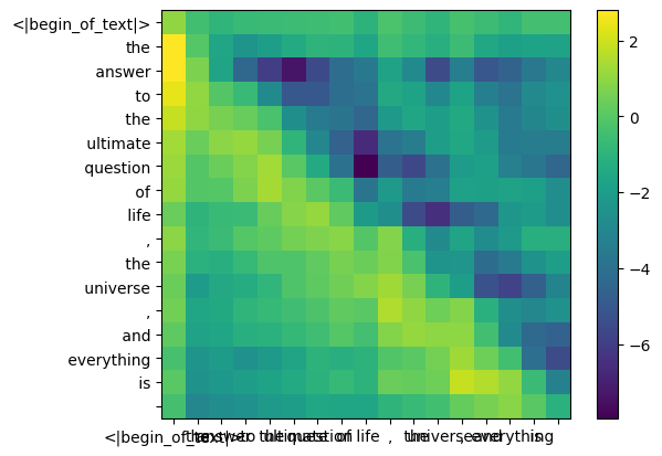
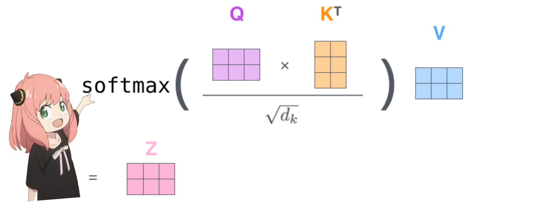
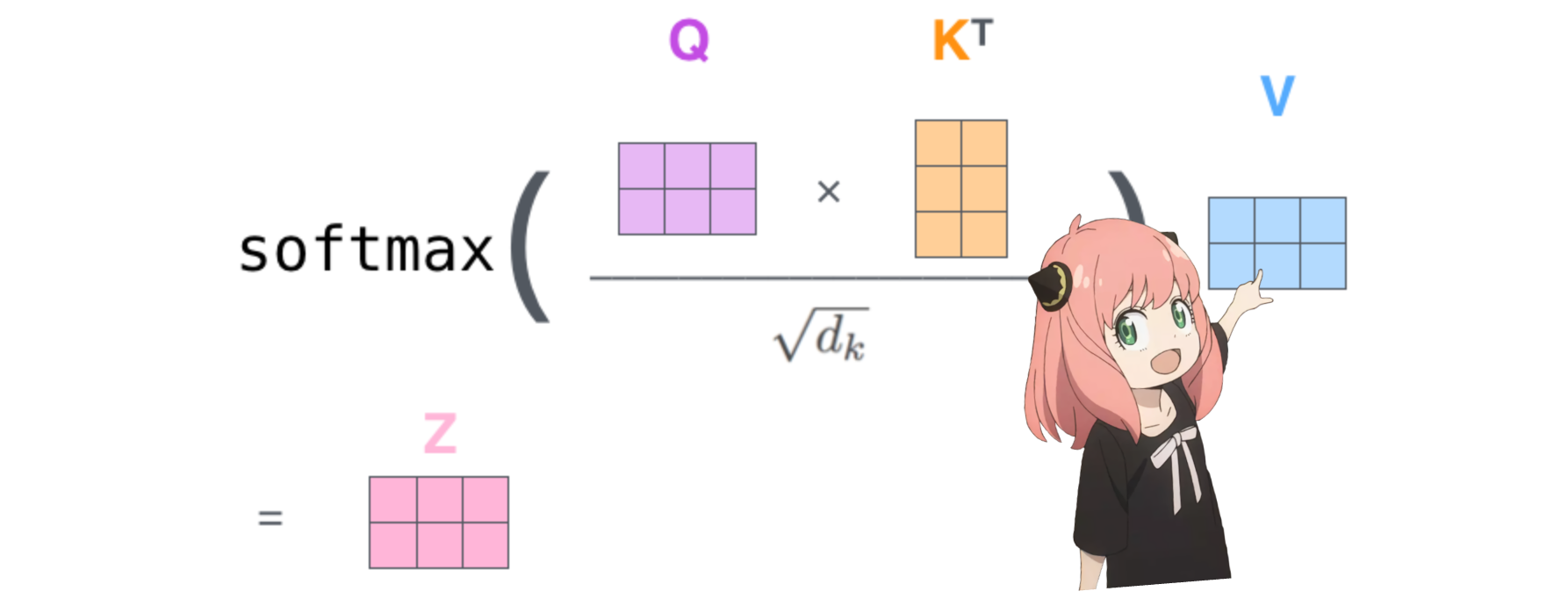
4.在下一步中，我们将乘以查询和关键矩阵

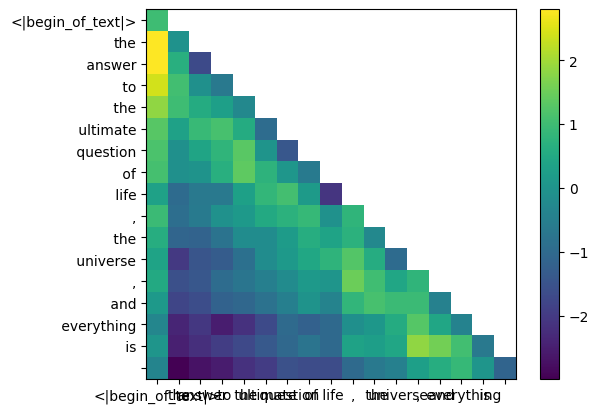
这样做将为我们提供一个将每个标记相互映射的分数，该分数描述了每个标记的查询与每个标记的密钥的相关程度。这是自我注意力 :) 注意力分数矩阵 (qk_per_token) 的形状是 [17x17]，其中 17 是提示中的标记数量

img

qk_per_token = torch.matmul(q_per_token_rotated, k_per_token_rotated.T)/(head_dim)**0.5
qk_per_token.shape
torch.Size([17, 17])

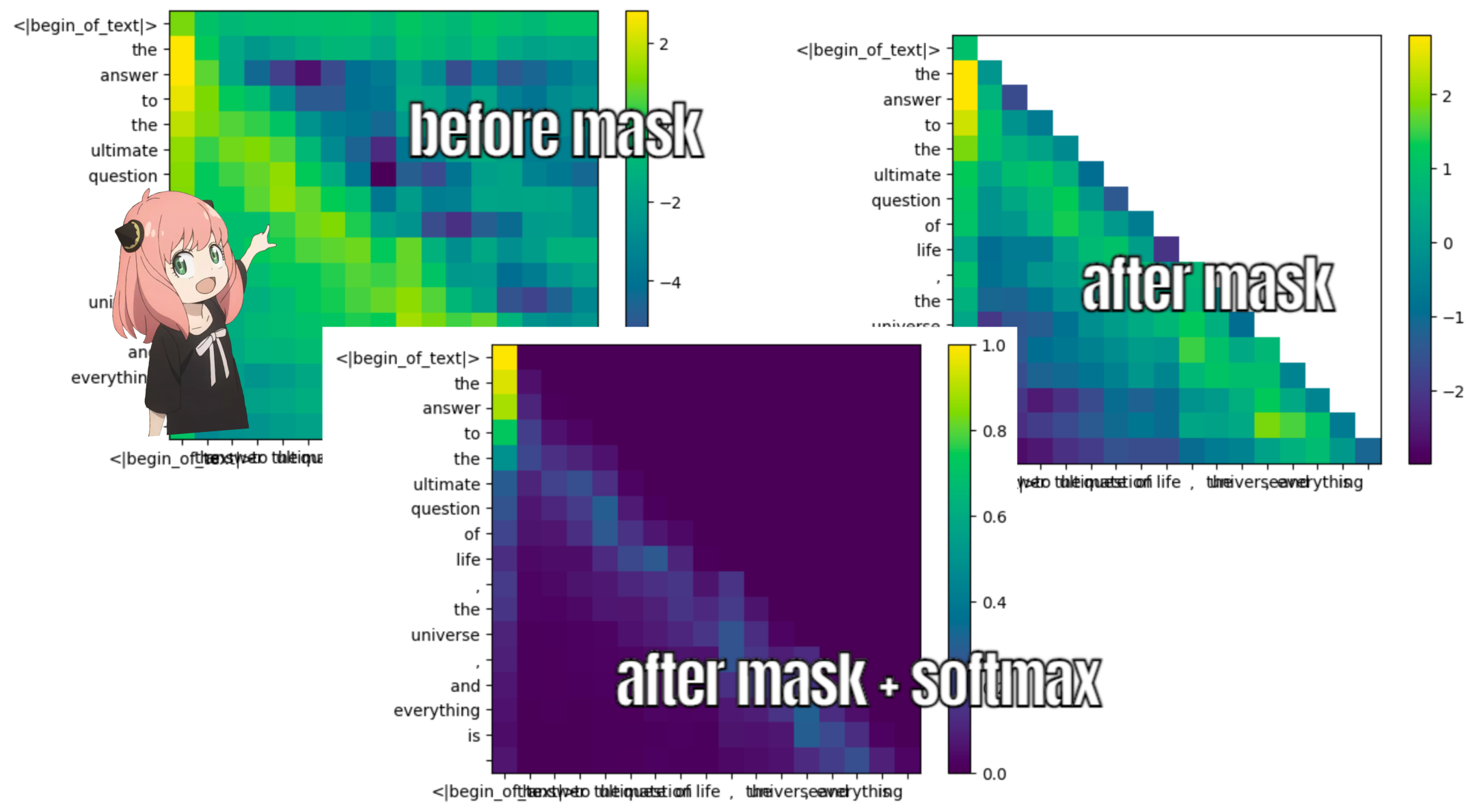
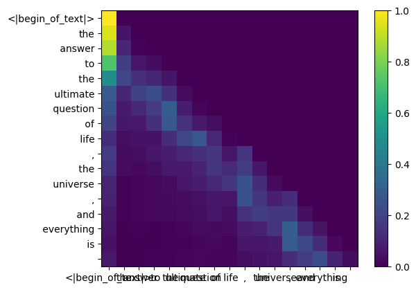
我们现在必须屏蔽查询关键分数

在 llama3 的训练过程中，未来的 token qk 分数被屏蔽。为什么？因为在训练期间我们只学习使用过去的标记来预测标记。 因此，在推理过程中，我们将未来的标记设置为零。

img

def display_qk_heatmap(qk_per_token):
    _, ax = plt.subplots()
    im = ax.imshow(qk_per_token.to(float).detach(), cmap='viridis')
    ax.set_xticks(range(len(prompt_split_as_tokens)))
    ax.set_yticks(range(len(prompt_split_as_tokens)))
    ax.set_xticklabels(prompt_split_as_tokens)
    ax.set_yticklabels(prompt_split_as_tokens)
    ax.figure.colorbar(im, ax=ax)
    
display_qk_heatmap(qk_per_token)

img

mask = torch.full((len(tokens), len(tokens)), float("-inf"), device=tokens.device)
mask = torch.triu(mask, diagonal=1)
mask
tensor([[0., -inf, -inf, -inf, -inf, -inf, -inf, -inf, -inf, -inf, -inf, -inf, -inf, -inf, -inf, -inf, -inf],
        [0., 0., -inf, -inf, -inf, -inf, -inf, -inf, -inf, -inf, -inf, -inf, -inf, -inf, -inf, -inf, -inf],
        [0., 0., 0., -inf, -inf, -inf, -inf, -inf, -inf, -inf, -inf, -inf, -inf, -inf, -inf, -inf, -inf],
        [0., 0., 0., 0., -inf, -inf, -inf, -inf, -inf, -inf, -inf, -inf, -inf, -inf, -inf, -inf, -inf],
        [0., 0., 0., 0., 0., -inf, -inf, -inf, -inf, -inf, -inf, -inf, -inf, -inf, -inf, -inf, -inf],
        [0., 0., 0., 0., 0., 0., -inf, -inf, -inf, -inf, -inf, -inf, -inf, -inf, -inf, -inf, -inf],
        [0., 0., 0., 0., 0., 0., 0., -inf, -inf, -inf, -inf, -inf, -inf, -inf, -inf, -inf, -inf],
        [0., 0., 0., 0., 0., 0., 0., 0., -inf, -inf, -inf, -inf, -inf, -inf, -inf, -inf, -inf],
        [0., 0., 0., 0., 0., 0., 0., 0., 0., -inf, -inf, -inf, -inf, -inf, -inf, -inf, -inf],
        [0., 0., 0., 0., 0., 0., 0., 0., 0., 0., -inf, -inf, -inf, -inf, -inf, -inf, -inf],
        [0., 0., 0., 0., 0., 0., 0., 0., 0., 0., 0., -inf, -inf, -inf, -inf, -inf, -inf],
        [0., 0., 0., 0., 0., 0., 0., 0., 0., 0., 0., 0., -inf, -inf, -inf, -inf, -inf],
        [0., 0., 0., 0., 0., 0., 0., 0., 0., 0., 0., 0., 0., -inf, -inf, -inf, -inf],
        [0., 0., 0., 0., 0., 0., 0., 0., 0., 0., 0., 0., 0., 0., -inf, -inf, -inf],
        [0., 0., 0., 0., 0., 0., 0., 0., 0., 0., 0., 0., 0., 0., 0., -inf, -inf],
        [0., 0., 0., 0., 0., 0., 0., 0., 0., 0., 0., 0., 0., 0., 0., 0., -inf],
        [0., 0., 0., 0., 0., 0., 0., 0., 0., 0., 0., 0., 0., 0., 0., 0., 0.]])
qk_per_token_after_masking = qk_per_token + mask
display_qk_heatmap(qk_per_token_after_masking)

img

img

qk_per_token_after_masking_after_softmax = torch.nn.functional.softmax(qk_per_token_after_masking, dim=1).to(torch.bfloat16)
display_qk_heatmap(qk_per_token_after_masking_after_softmax)

img

值（values）（注意力几乎结束）

img

这些分数（0-1）用于确定每个标记使用了多少值矩阵 >就像键一样，值权重也每4个注意力头共享（以节省计算） >因此，值的形状下面的权重矩阵是[8x128x4096]

v_layer0 = model["layers.0.attention.wv.weight"]
v_layer0 = v_layer0.view(n_kv_heads, v_layer0.shape[0] // n_kv_heads, dim)
v_layer0.shape
torch.Size([8, 128, 4096])

下面给出第一层第一头值权重矩阵

v_layer0_head0 = v_layer0[0]
v_layer0_head0.shape
torch.Size([128, 4096])

值向量（value vectors）

img

我们现在使用值权重来获取每个标记的注意力值，其大小为 [17x128]，其中 17 是提示中标记的数量，128 是每个标记的值向量的暗度

v_per_token = torch.matmul(token_embeddings, v_layer0_head0.T)
v_per_token.shape
torch.Size([17, 128])

5.注意力

img

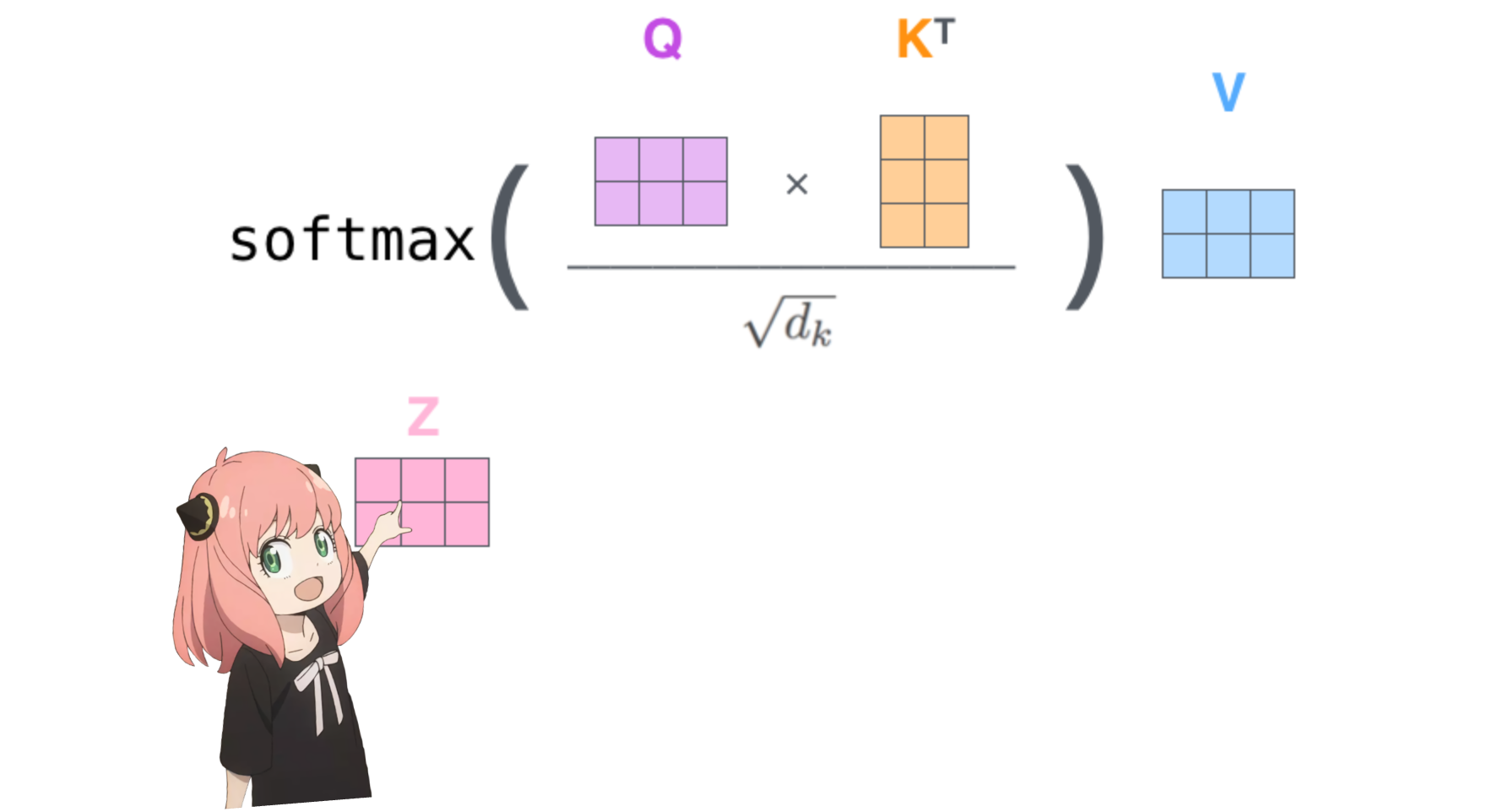
与每个标记的值相乘后得到的注意力向量的形状为 [17*128]

qkv_attention = torch.matmul(qk_per_token_after_masking_after_softmax, v_per_token)
qkv_attention.shape
torch.Size([17, 128])

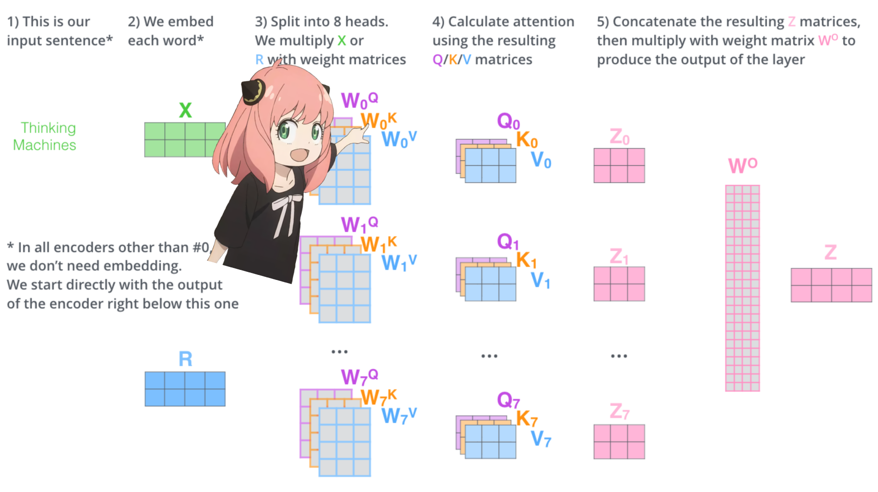
多头注意力

我们现在有了第一层和第一个头的注意力值， 现在我将运行一个循环并执行与上面的单元完全相同的数学运算，但对于第一层中的每个头

qkv_attention_store = []

for head in range(n_heads):
    q_layer0_head = q_layer0[head]
    k_layer0_head = k_layer0[head//4] # key weights are shared across 4 heads
    v_layer0_head = v_layer0[head//4] # value weights are shared across 4 heads
    q_per_token = torch.matmul(token_embeddings, q_layer0_head.T)
    k_per_token = torch.matmul(token_embeddings, k_layer0_head.T)
    v_per_token = torch.matmul(token_embeddings, v_layer0_head.T)

    q_per_token_split_into_pairs = q_per_token.float().view(q_per_token.shape[0], -1, 2)
    q_per_token_as_complex_numbers = torch.view_as_complex(q_per_token_split_into_pairs)
    q_per_token_split_into_pairs_rotated = torch.view_as_real(q_per_token_as_complex_numbers * freqs_cis[:len(tokens)])
    q_per_token_rotated = q_per_token_split_into_pairs_rotated.view(q_per_token.shape)

    k_per_token_split_into_pairs = k_per_token.float().view(k_per_token.shape[0], -1, 2)
    k_per_token_as_complex_numbers = torch.view_as_complex(k_per_token_split_into_pairs)
    k_per_token_split_into_pairs_rotated = torch.view_as_real(k_per_token_as_complex_numbers * freqs_cis[:len(tokens)])
    k_per_token_rotated = k_per_token_split_into_pairs_rotated.view(k_per_token.shape)

    qk_per_token = torch.matmul(q_per_token_rotated, k_per_token_rotated.T)/(128)**0.5
    mask = torch.full((len(tokens), len(tokens)), float("-inf"), device=tokens.device)
    mask = torch.triu(mask, diagonal=1)
    qk_per_token_after_masking = qk_per_token + mask
    qk_per_token_after_masking_after_softmax = torch.nn.functional.softmax(qk_per_token_after_masking, dim=1).to(torch.bfloat16)
    qkv_attention = torch.matmul(qk_per_token_after_masking_after_softmax, v_per_token)
    qkv_attention = torch.matmul(qk_per_token_after_masking_after_softmax, v_per_token)
    qkv_attention_store.append(qkv_attention)

len(qkv_attention_store)
32

img

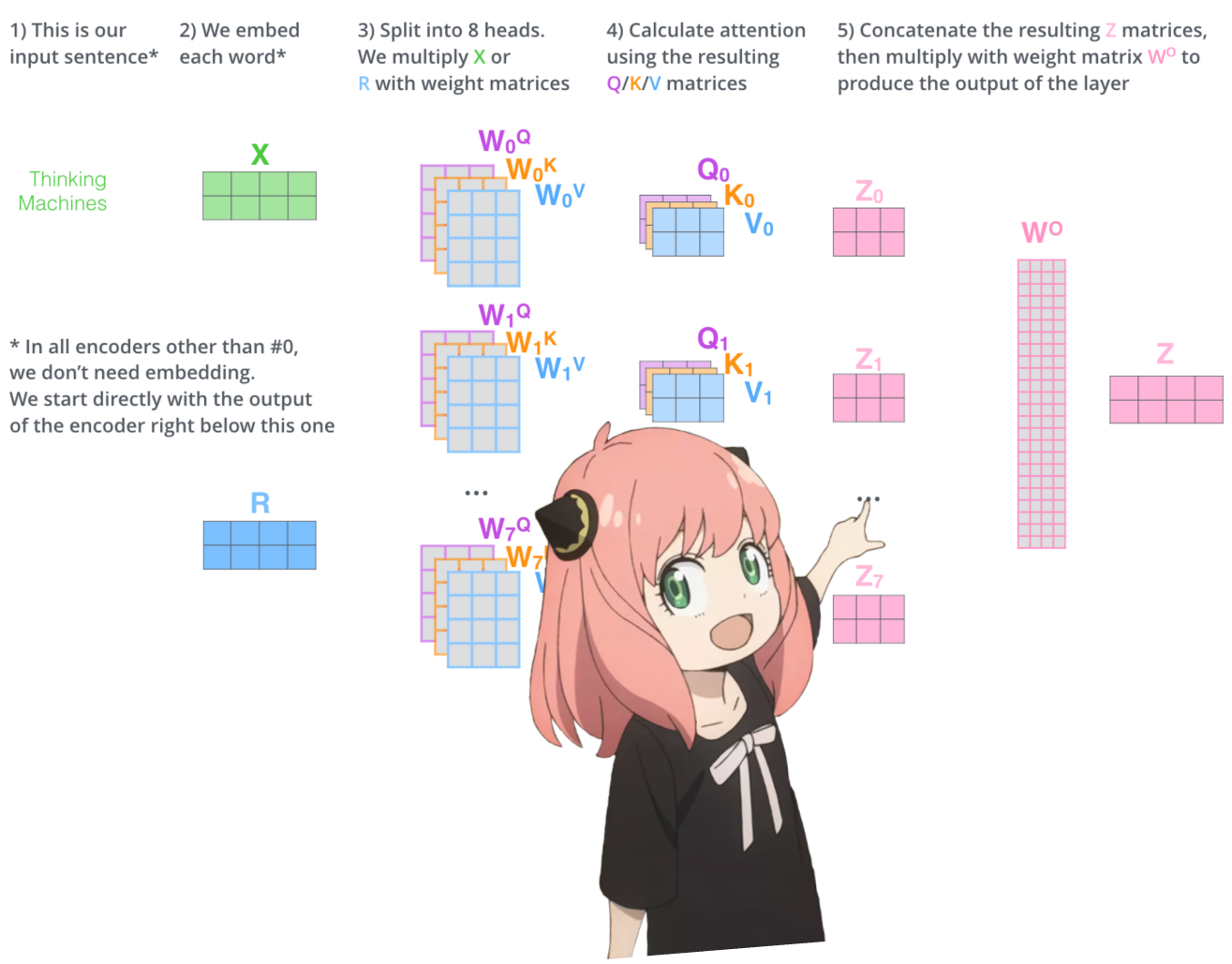
我们现在有了第一层所有 32 个头的 qkv_attention 矩阵，接下来我将把所有注意力分数合并到一个大小为 [17x4096] 的大矩阵中， 我们即将结束:)

stacked_qkv_attention = torch.cat(qkv_attention_store, dim=-1)
stacked_qkv_attention.shape
torch.Size([17, 4096])

6.权重矩阵，最后步骤之一

img

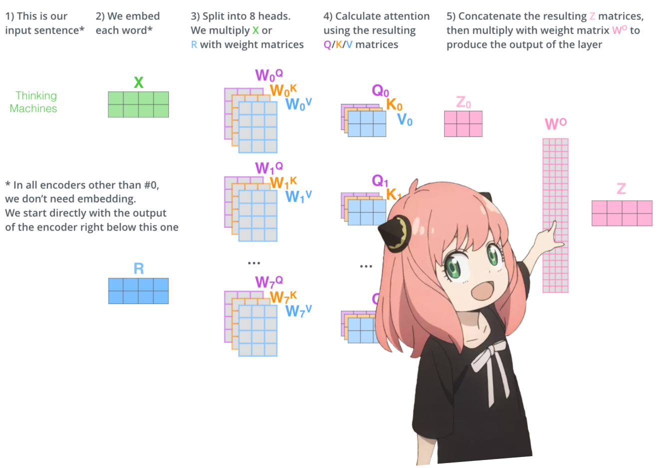
对于第 0 层注意力要做的最后一件事是乘以

w_layer0 = model["layers.0.attention.wo.weight"]
w_layer0.shape
torch.Size([4096, 4096])

这是一个简单的线性层，所以我们只需 matmul

embedding_delta = torch.matmul(stacked_qkv_attention, w_layer0.T)
embedding_delta.shape
torch.Size([17, 4096])

img

我们现在在注意力之后嵌入值发生了变化，这应该添加到原始令牌嵌入中

embedding_after_edit = token_embeddings_unnormalized + embedding_delta
embedding_after_edit.shape
torch.Size([17, 4096])

7.我们进行标准化，然后通过嵌入增量运行前馈神经网络

img

embedding_after_edit_normalized = rms_norm(embedding_after_edit, model["layers.0.ffn_norm.weight"])
embedding_after_edit_normalized.shape
torch.Size([17, 4096])

加载 ff 权重并实现前馈网络

img

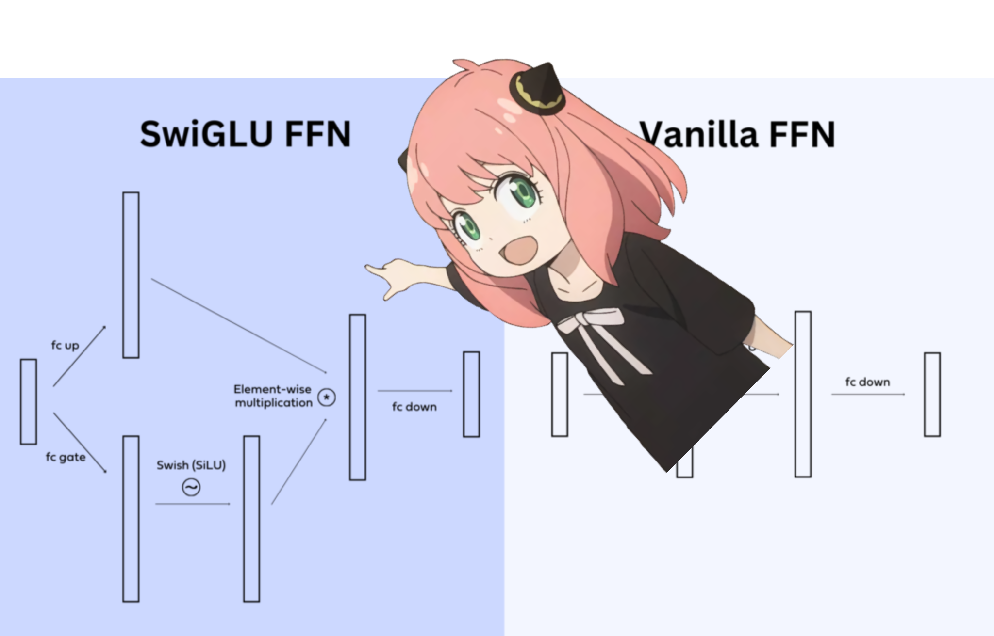
在 llama3 中，他们使用了 SwiGLU 前馈网络，这种网络架构非常擅长在模型需要时添加非线性。 如今在 llms 中使用这种前馈网络架构是相当标准的

w1 = model["layers.0.feed_forward.w1.weight"]
w2 = model["layers.0.feed_forward.w2.weight"]
w3 = model["layers.0.feed_forward.w3.weight"]
output_after_feedforward = torch.matmul(torch.functional.F.silu(torch.matmul(embedding_after_edit_normalized, w1.T)) * torch.matmul(embedding_after_edit_normalized, w3.T), w2.T)
output_after_feedforward.shape
torch.Size([17, 4096])

我们终于在第一层之后为每个令牌有了新编辑的嵌入

在我们完成之前还需要 31 层（一个 for 循环）， 您可以想象这个编辑后的嵌入包含有关第一层上提出的所有查询的信息， 现在每一层都会对所提出的问题编码越来越复杂的查询，直到我们有一个嵌入知道我们需要的下一个令牌的所有信息。

layer_0_embedding = embedding_after_edit+output_after_feedforward
layer_0_embedding.shape
torch.Size([17, 4096])

天哪，一切都同时发生

img

是的，就是这样。我们之前为每一层所做的一切都是一次性完成的。

祝阅读愉快:)

final_embedding = token_embeddings_unnormalized
for layer in range(n_layers):
    qkv_attention_store = []
    layer_embedding_norm = rms_norm(final_embedding, model[f"layers.{layer}.attention_norm.weight"])
    q_layer = model[f"layers.{layer}.attention.wq.weight"]
    q_layer = q_layer.view(n_heads, q_layer.shape[0] // n_heads, dim)
    k_layer = model[f"layers.{layer}.attention.wk.weight"]
    k_layer = k_layer.view(n_kv_heads, k_layer.shape[0] // n_kv_heads, dim)
    v_layer = model[f"layers.{layer}.attention.wv.weight"]
    v_layer = v_layer.view(n_kv_heads, v_layer.shape[0] // n_kv_heads, dim)
    w_layer = model[f"layers.{layer}.attention.wo.weight"]
    for head in range(n_heads):
        q_layer_head = q_layer[head]
        k_layer_head = k_layer[head//4]
        v_layer_head = v_layer[head//4]
        q_per_token = torch.matmul(layer_embedding_norm, q_layer_head.T)
        k_per_token = torch.matmul(layer_embedding_norm, k_layer_head.T)
        v_per_token = torch.matmul(layer_embedding_norm, v_layer_head.T)
        q_per_token_split_into_pairs = q_per_token.float().view(q_per_token.shape[0], -1, 2)
        q_per_token_as_complex_numbers = torch.view_as_complex(q_per_token_split_into_pairs)
        q_per_token_split_into_pairs_rotated = torch.view_as_real(q_per_token_as_complex_numbers * freqs_cis)
        q_per_token_rotated = q_per_token_split_into_pairs_rotated.view(q_per_token.shape)
        k_per_token_split_into_pairs = k_per_token.float().view(k_per_token.shape[0], -1, 2)
        k_per_token_as_complex_numbers = torch.view_as_complex(k_per_token_split_into_pairs)
        k_per_token_split_into_pairs_rotated = torch.view_as_real(k_per_token_as_complex_numbers * freqs_cis)
        k_per_token_rotated = k_per_token_split_into_pairs_rotated.view(k_per_token.shape)
        qk_per_token = torch.matmul(q_per_token_rotated, k_per_token_rotated.T)/(128)**0.5
        mask = torch.full((len(token_embeddings_unnormalized), len(token_embeddings_unnormalized)), float("-inf"))
        mask = torch.triu(mask, diagonal=1)
        qk_per_token_after_masking = qk_per_token + mask
        qk_per_token_after_masking_after_softmax = torch.nn.functional.softmax(qk_per_token_after_masking, dim=1).to(torch.bfloat16)
        qkv_attention = torch.matmul(qk_per_token_after_masking_after_softmax, v_per_token)
        qkv_attention_store.append(qkv_attention)

    stacked_qkv_attention = torch.cat(qkv_attention_store, dim=-1)
    w_layer = model[f"layers.{layer}.attention.wo.weight"]
    embedding_delta = torch.matmul(stacked_qkv_attention, w_layer.T)
    embedding_after_edit = final_embedding + embedding_delta
    embedding_after_edit_normalized = rms_norm(embedding_after_edit, model[f"layers.{layer}.ffn_norm.weight"])
    w1 = model[f"layers.{layer}.feed_forward.w1.weight"]
    w2 = model[f"layers.{layer}.feed_forward.w2.weight"]
    w3 = model[f"layers.{layer}.feed_forward.w3.weight"]
    output_after_feedforward = torch.matmul(torch.functional.F.silu(torch.matmul(embedding_after_edit_normalized, w1.T)) * torch.matmul(embedding_after_edit_normalized, w3.T), w2.T)
    final_embedding = embedding_after_edit+output_after_feedforward

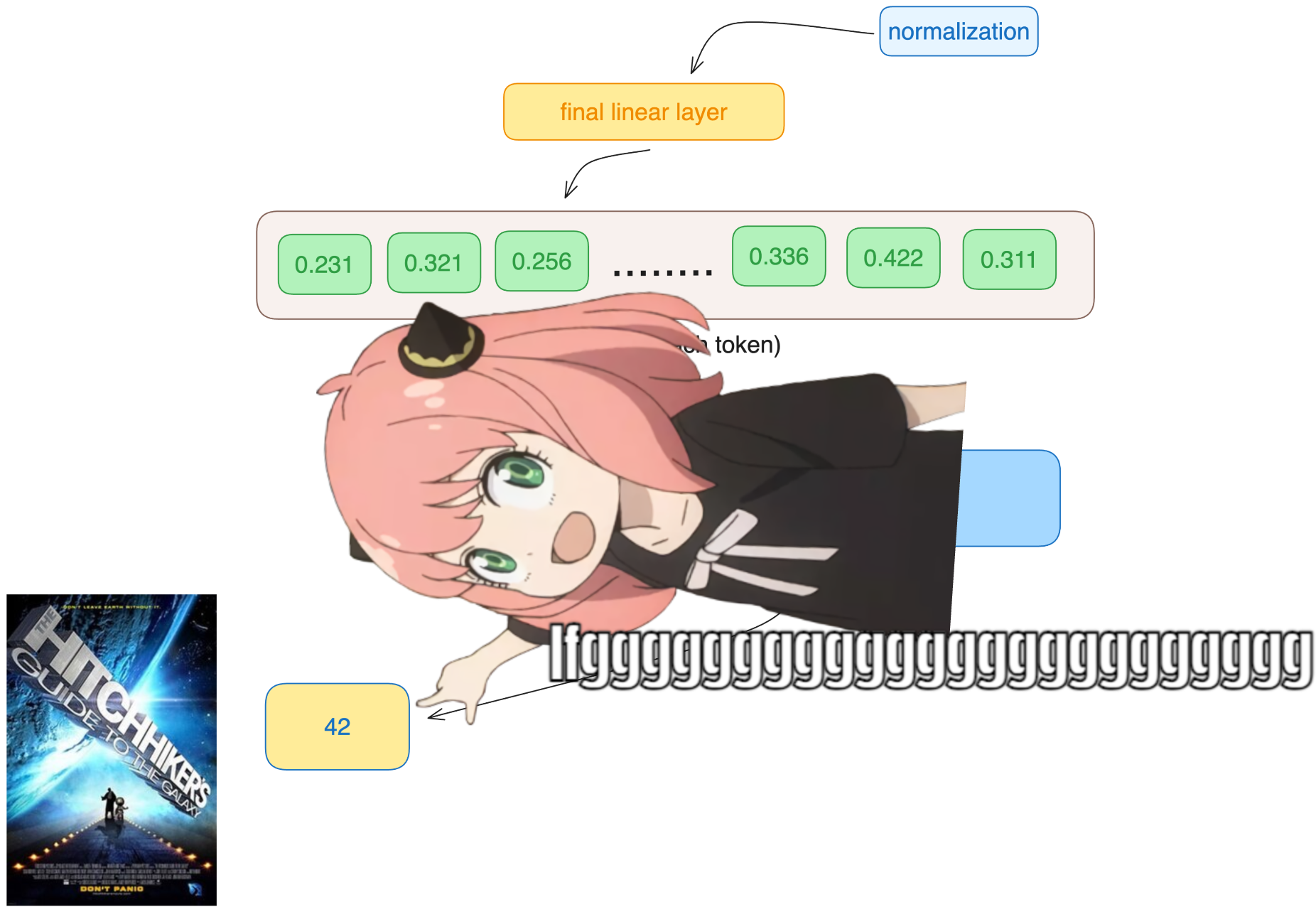
8.我们现在有了最终的嵌入，模型可以对下一个标记做出的最佳猜测

嵌入的形状与常规令牌嵌入 [17x4096] 相同，其中 17 是令牌数量，4096 是嵌入暗淡

img

final_embedding = rms_norm(final_embedding, model["norm.weight"])
final_embedding.shape
torch.Size([17, 4096])

最后，让我们将嵌入解码到令牌值中

img

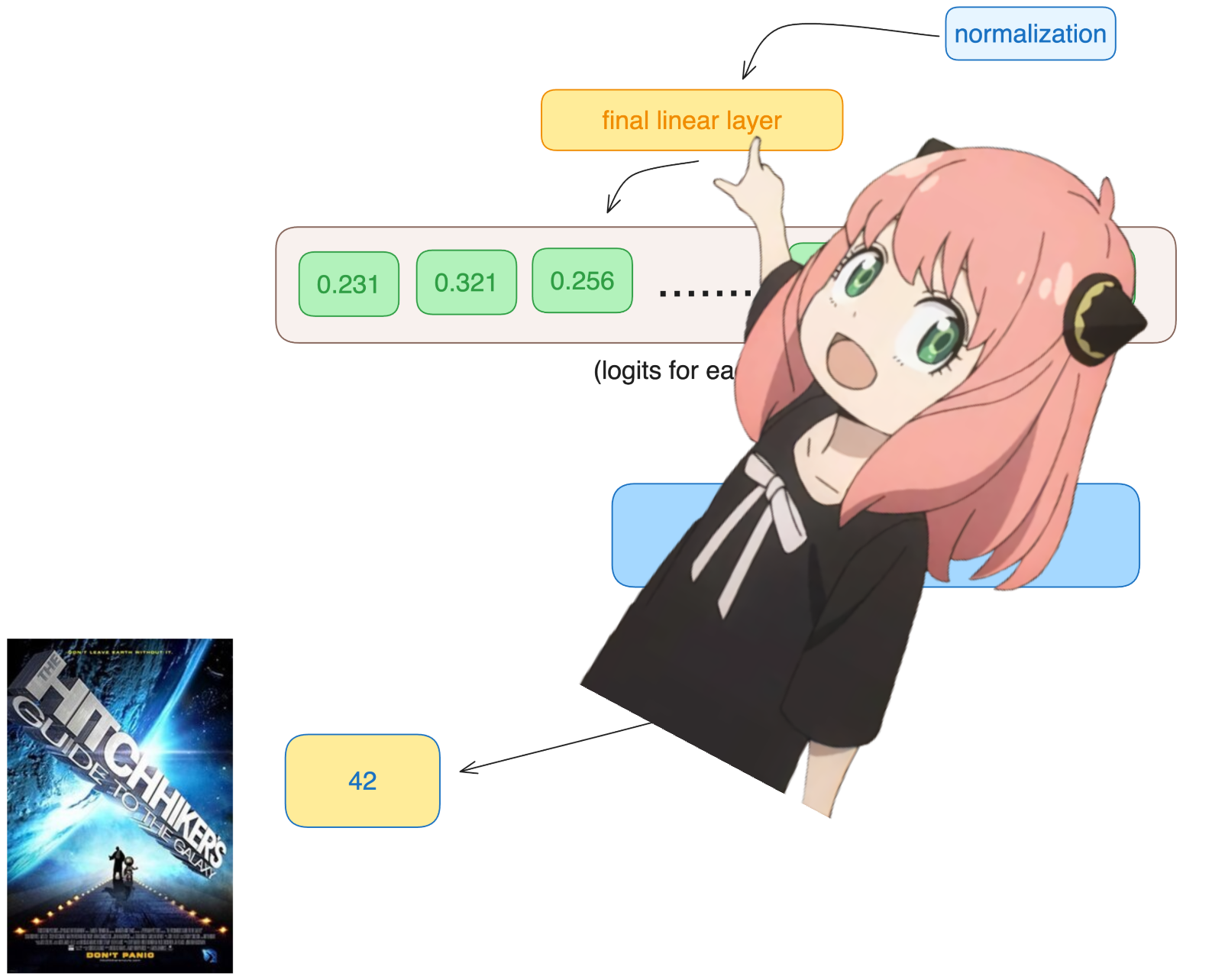
我们将使用输出解码器将最终的嵌入转换为令牌

model["output.weight"].shape
torch.Size([128256, 4096])

我们使用最后一个标记的嵌入来预测下一个值

希望在我们的例子中，42 :) 注意：42 是“生命、宇宙和一切的终极问题的答案”的答案，根据《银河系漫游指南》一书，大多数现代 llms 都会回答这里有 42，这应该验证我们的整个代码！祝我好运 ：）

logits = torch.matmul(final_embedding[-1], model["output.weight"].T)
logits.shape
torch.Size([128256])

模型预测令牌编号 2983 作为下一个令牌，这是 42 的令牌编号吗？

我正在向您宣传，这是代码的最后一个单元格，希望您玩得开心:)

next_token = torch.argmax(logits, dim=-1)
next_token
tensor(2983)

Let's go

img

tokenizer.decode([next_token.item()])
#输出'42'